This guide will describe how you go from Excel to app, and you will learn how Molnify reads your Excel file as an instruction for how Molnify should create your app. Important things such as how you can structure your Excel model, which colors to use for inputs and outputs, and in what way Molnify reads the Excel file will be described. This is a simple guide, created to give you an understanding of how you build Molnify apps and to provide you with the basic knowledge so that you can build your own apps quickly and easily.

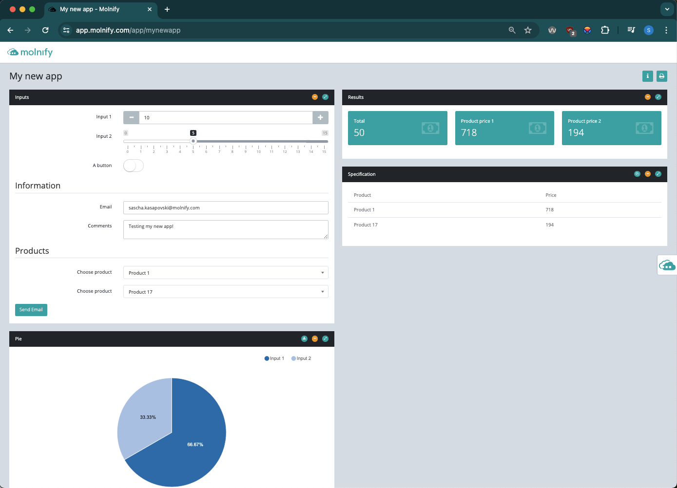
Below you can see the app that we are going to create. The app itself has no real use case and the purpose is to show you the ropes when it comes to Molnify app development and what you can do with Molnify with little bit of imagination. You can try out the app by clicking this link: https://app.molnify.com/app/mynewapp.

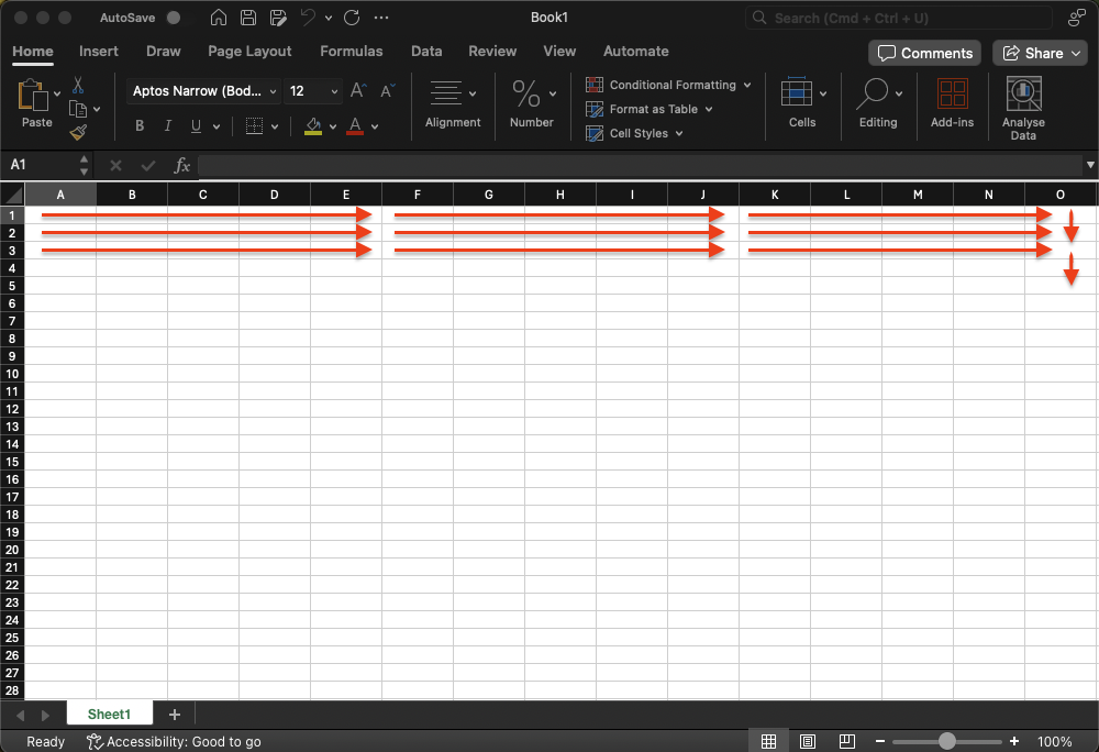
To begin with, how does Molnify read the Excel file? Well, from left to right, from top to bottom.

In this guide, we will talk about inputs (green cells), outputs (red cells), charts and tables (blue cells), actions (yellow cells), and metadata (purple cells).

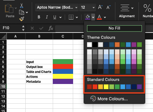
It is important that you only use the standard colors of Excel or Google Sheets. For inputs, it is green, not light green or dark green, that applies.

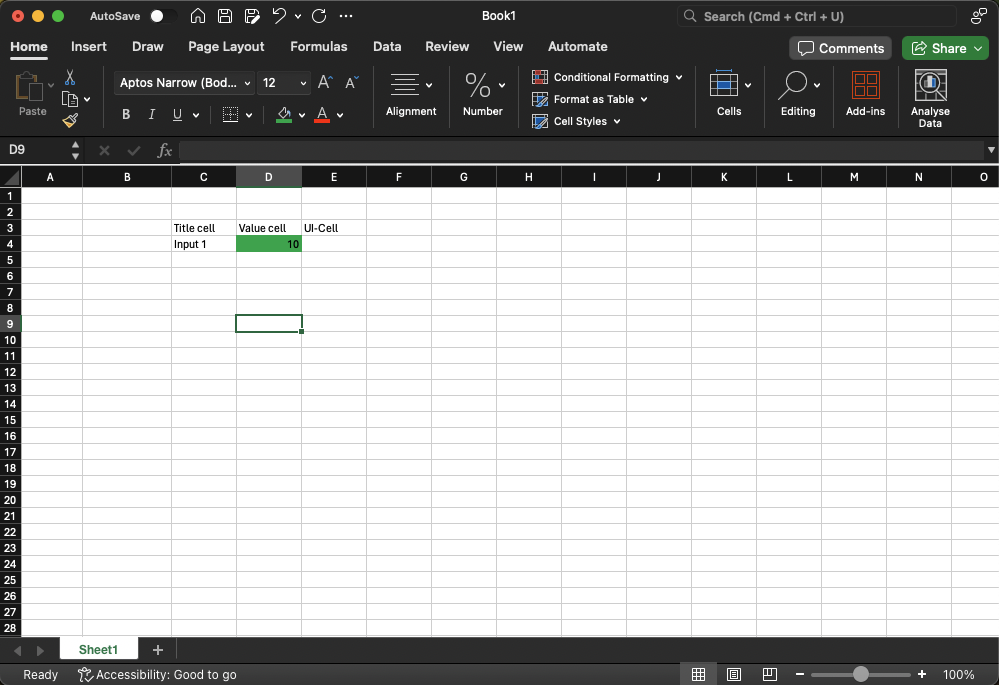
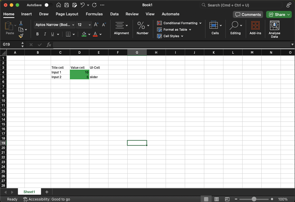
To build an input, it requires three consecutive cells in your Excel file: a title cell, a value cell (green cell), and a UI cell. You do not need to write anything in the UI cell, but it needs its place. In the example below, for instance, you would not be able to have a new title cell in column E, which is Input 1's UI cell.

Now let's add another input. We can add this on the same row, in columns F, G, and H, or we can put it on the next row. Since Molnify reads the file from left to right, top to bottom, both options would result in this becoming the next inputs. Now we will also add slider in the UI cell, which will make input 2 a slider when the file is uploaded and used as an app.

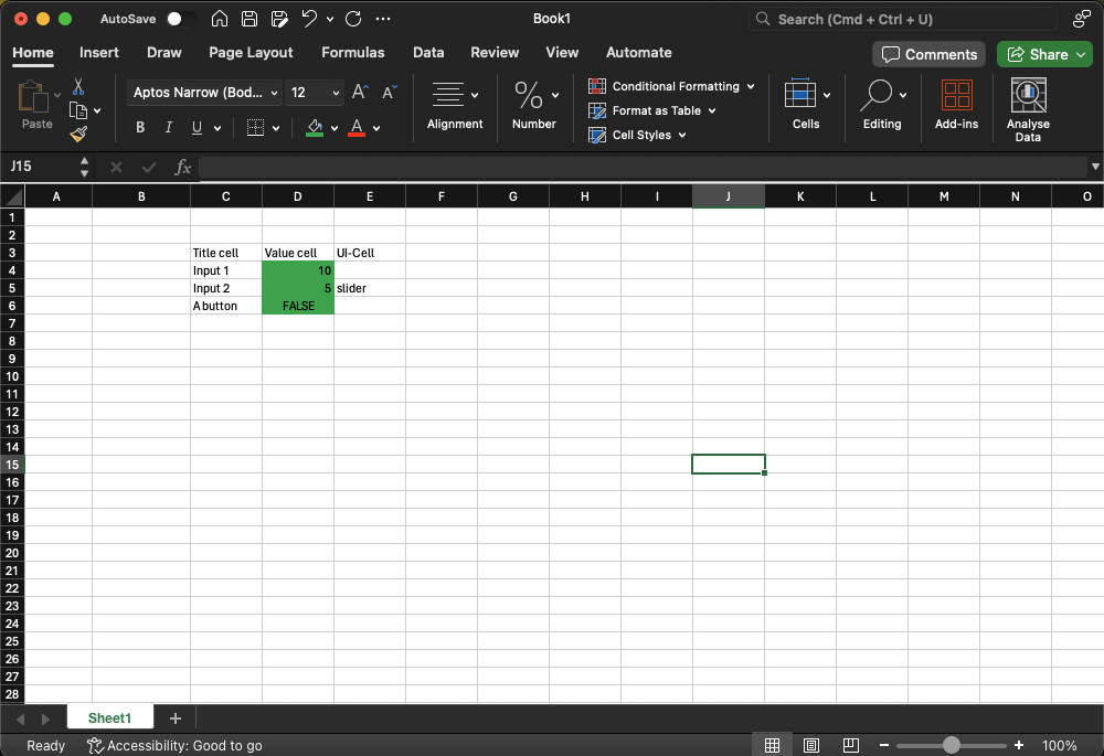
We are now going to add a button. TRUE and FALSE become clickable buttons in Molnify. We will make this the third input, so for simplicity's sake, we will just place it on the next row.

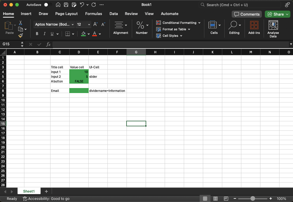
Now we also want to create a simple text box, where the app user can write their email. To separate this part in the app, we will use the UI cell command dividername=Information,” to create a divider line, and a slightly larger text that reads “Information.”

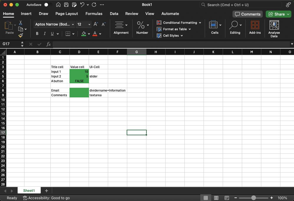
Under this input, we want to have a slightly larger text box where a user of the app can write a bit longer text. We use the UI cell command textarea.

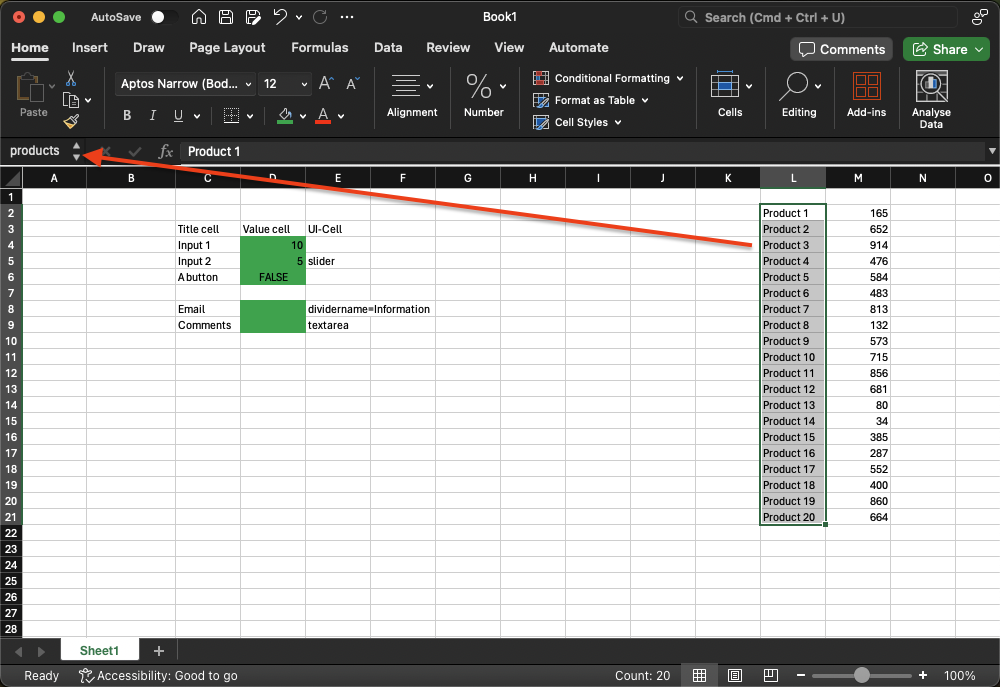
We will now add a list of products in our app. We do this by listing product 1 to 20 and in the next column we add various prices. To have a list in the app, we convert the cells where it says product 1 to 20 into a named range and name it products:

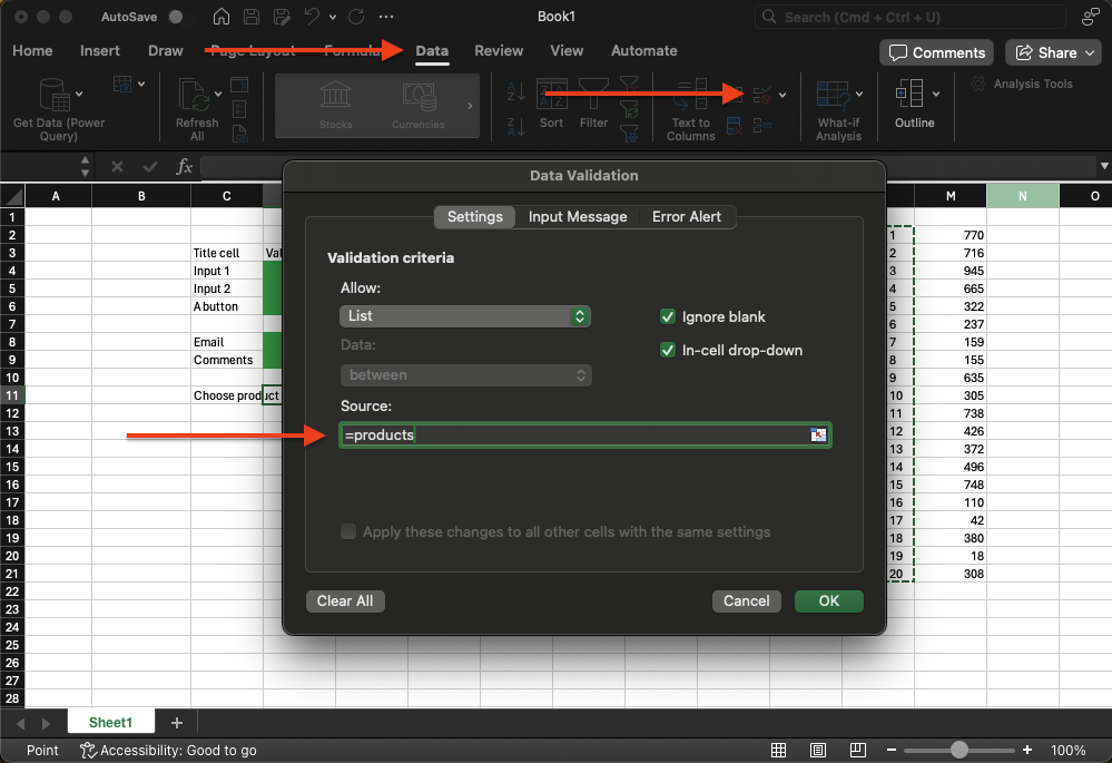
We then create the input by coming up with a title, and in the value cell go to Data and Data Validation and then choose “List” and enter =products. Note that you must use a named range for this, it does not work to have cell references or formulas here.

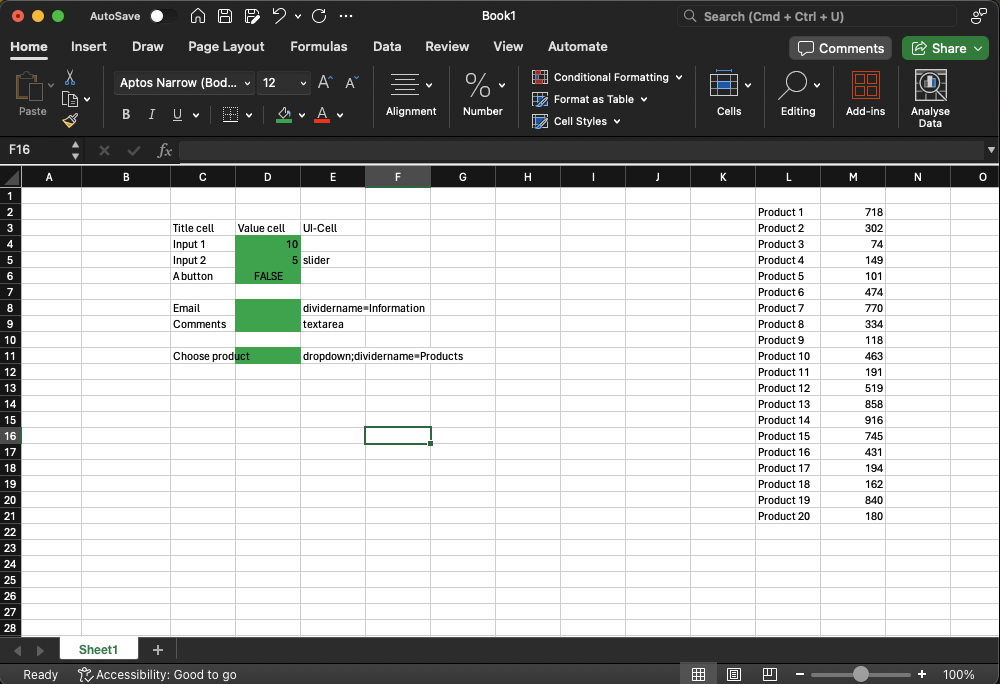
We then color the value cell green, write dropdown in the UI cell, and we also add a dividername=Products. To separate the two UI commands dropdown and dividername=, we use a semicolon ;. You can write many different UI cell commands in the same UI cell and you always separate them by putting a semicolon between them.

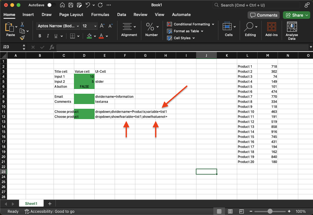
Now we imagine that as soon as someone has chosen a product in the list, we want a new input, with a new list to be shown. This next input should thus be hidden as long as a choice has not been made in list number 1. We can hide or show inputs (and outputs) by using conditional show. For the conditional show to know which input to look at, we give the first list a name by writing in its UI cell: ;variable=list1 We then simply copy the title and value cell from row 11 and paste into row 12. We add dropdown and the conditional show command: showifvariable=list1 so Molnify knows what to monitor and then, after a semicolon, showifvaluenot= (i.e., show if the value in the variable list one is not nothing).

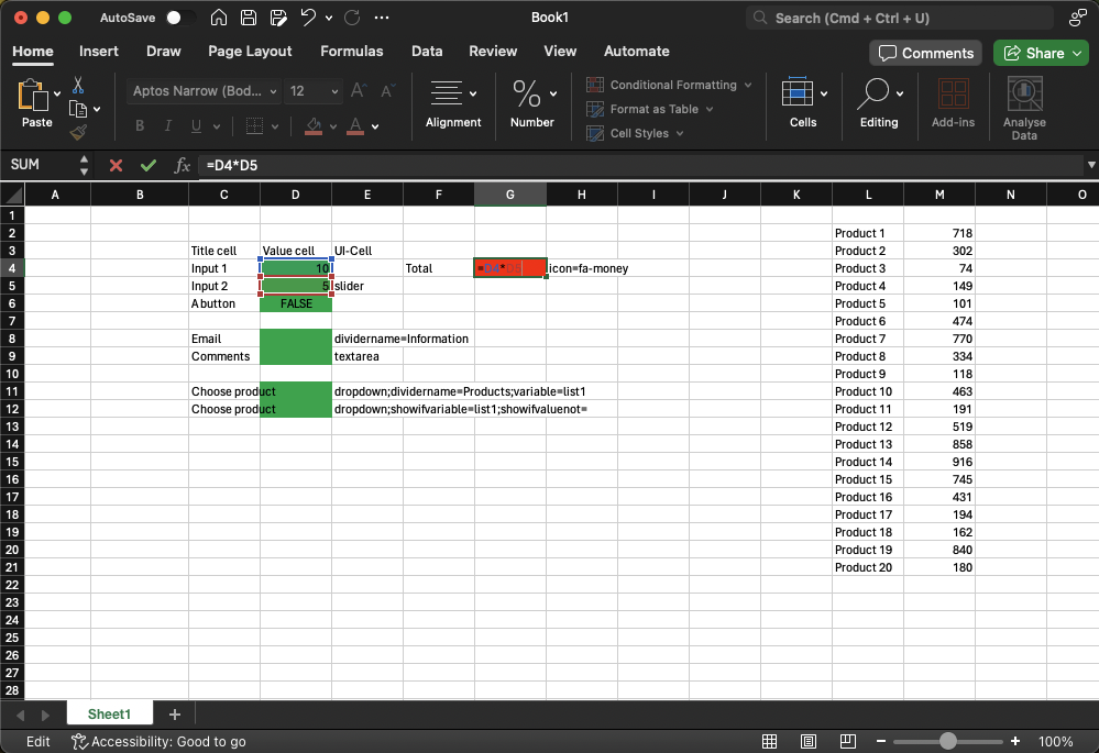
Now we will build three output boxes. One that shows Input 1 * Input 2, one that shows the price of Product 1, and one that shows the price of Product 2.

To build the first output, we need: Title cell, value cell (red) and UI cell, just like with inputs. We write Total as the title, create a simple Excel formula =D4*D5 in the next cell which we color red and in the UI cell we write icon=fa-money (Molnify uses the Font Awesome 4.7 library for icons).

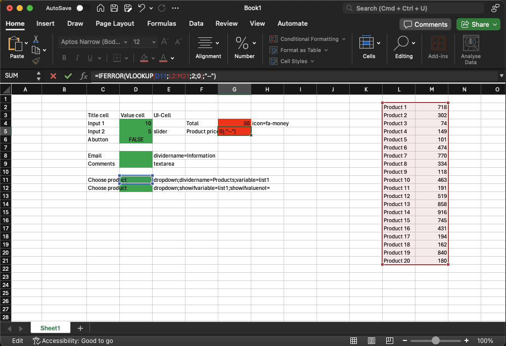
The next output becomes a bit more advanced and here we will create a =VLOOKUP function that searches our product list for the price of the product selected in the first list. Since initially there will be no choice made in the list, this formula will return N/A and we do not want to see that. Therefore, we create a =IFERROR function around the =VLOOKUP so that as long as no result exists, two dashes are displayed. The formula therefore looks like this: =IFERROR(VLOOKUP(D11;L2:M21;2;0);"--")

We give the output a title, Product 1, and then color the cell with our formula in red. This time we skip the UI cell.

For the output Product 2, we simply repeat what we did to create the previous output:

Now we will create a table. Tables are blue cells and, like inputs and outputs, have a title cell and a UI cell. Your table also has column titles. A table can contain several value cells in a row, as well as several rows. If all cells in a row have the value “” i.e., two quotation marks, that row will be hidden. This is useful if, for example, you want a table where more rows are shown only after more selections have been made in the app, and remain hidden until then. In our table, we will display the product name and the price of the product for product 1 on one row, and product 2 on the next row. We will name the table Specification. In the table's UI cell, we will write table. The table will have two rows, so we create a title cell, column titles, blue cells for the table's content, and a UI cell first. We will add the formulas later.

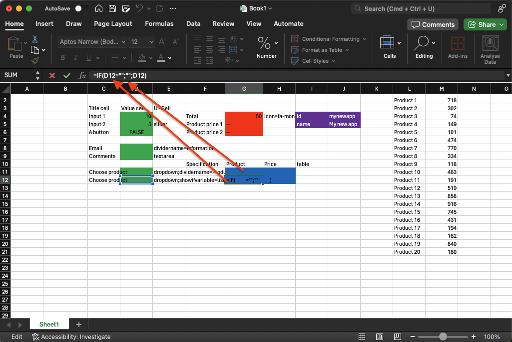
Now let's fix the formulas: An IF formula that looks at the green cell for product 1. If no choice is made, show “” and if a choice is made, display what is in the cell where the list is. We then simply drag the formula down to the row below.

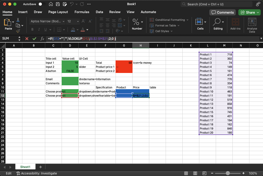
In the two other columns, we want to display the price, but hide it if no choice is made. The formulas will thus be in cell H11: =IF(G11="";"";VLOOKUP(D11;$L$2:$M$21;2;0)) and for H12 we can just drag down the formula so it becomes: =IF(G12="";"";VLOOKUP(D12;$L$2:$M$21;2;0))

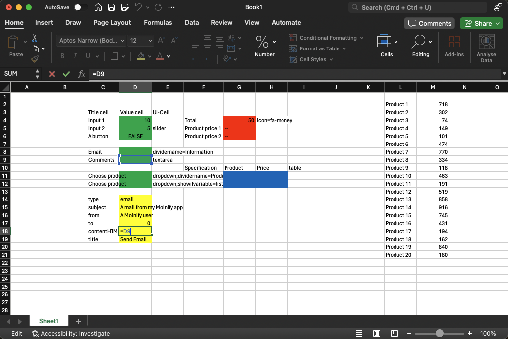
Now we will create a super simple email action, with yellow cells! We want an action that takes what is written in cell D9 (i.e., the comment) and sends this in an email to the email address entered in cell D8.

To create an email action, we write:

• type and then in the next cell to the right (yellow cell) email
• subject and then in the next cell to the right (yellow cell) An email from my Molnify app
• from and then in the next cell to the right (yellow cell) A Molnify user (we could have used a cell reference, a name, or similar here)
• to and then in the next cell to the right (yellow cell) =D8
• contentHTML and then in the next cell to the right (yellow cell) =D9
• title and then in the next cell to the right (yellow cell) Send email

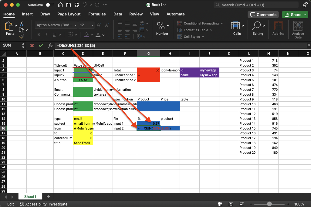
We will now create another output - a pie chart. Charts, just like tables, are blue cells in Molnify. A chart can have several rows and columns, but a pie chart can only have several rows and one column. We make this chart in the simplest possible way. We set the title cell to Pie, as a column title we write a % sign, and in the UI cell, we write piechart. As titles for the rows that will have blue value cells, we make cell references to C4 and C5, so the titles become Input 1 and Input 2. In the top blue cell, we write the following formula: =D4/SUM($D$4:$D$5) then we drag the formula down to the next row and get the following: =D5/SUM($D$4:$D$5)

We reduce the decimals in both cells and we now have two cells that sum up to 1. Perfect for a pie chart!

Now it's time for metadata (purple cells). Metadata, unlike inputs and outputs as well as actions, require that all cells that are metadata are colored purple. In the metadata, we will set the id of the app, which also becomes the end of the app URL, and name, which becomes the name of the app. There are many more meta commands that, for example, style the app, set user restrictions on the app and even metadata where you can write SQL strings that operate on Molnify's SQL database. But, in this guide, we keep it simple and are satisfied with id and name.

So, in cells that we color purple, we write id and then in the next cell that is purple mynewapp. If you follow this guide and build your own app, change "mynewapp" to something else, since I have already uploaded an app with the id "mynewapp". If you upload a file with an id that is already taken, Molnify will make up an id for you, which you have not chosen. A difference will also be that if you make changes to your app and upload the file again with an id that is already taken, Molnify creates a copy, with a new invented id. On the other hand, if you have written an id that does not exist, you will 1, get to keep your own id and 2, when you update by uploading the file again, not create a new copy of the app, but simply replace your old app with your new one.

We also enter name followed by My new app in the next purple cell to the right.

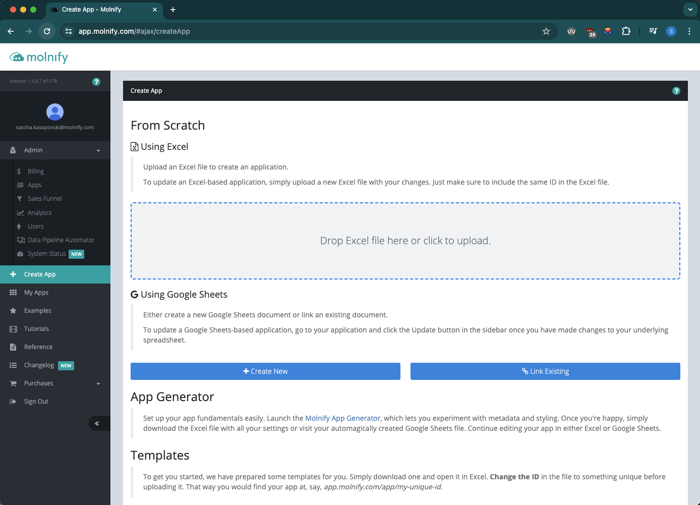
We then go to app.molnify.com and click on Create app. We take our Excel file and drop it over the area that says Drop Excel file here or click to upload.

Now Molnify reads the Excel file as an instruction for how the app should be built and after a few seconds, the app is ready to be used. In our case, the URL becomes https://app.molnify.com/app/mynewapp but in your case, you have probably chosen another id, so the end of your URL will be something else. This is what the app looks like when it has become an app:

If you want to continue developing your app, you make changes to your Excel file, add inputs and outputs, save your Excel file on your computer (a good idea is to save the file with different names, so you can go back to a previous version if something goes wrong). When you want to upload a new version, you don't need to go back to app.molnify.com and click on Create app, but you can instead click out the sidebar in your app (it's just you who uploads that sees it, as well as any Managers or SuperUsers that you have defined in your metadata) and here you can drop new versions of your Excel model, so the app gets updated.

This was a simple guide to help you get started. There are many more functions in Molnify and if you want to read about them, you can do so in our Reference Guide. You can also check out our YouTube channel, where we have several video tutorials that show guides like this, but also more advanced tutorials for other functions.

You can download the Excel file that forms the basis for this app if you want to experiment or use it as a basis for your own app.

Enjoy building your app and if you have questions you can always email info@molnify.com or if you want personal guidance you can book a meeting with us.